“Action speak louder than words. ”
[TOC]
1 构建一个基于感知机的手写数字识别神经网络
对感知机不了解的可以看之前博客《统计学习方法》(李航)读书笔记(二)
1.1 什么是神经网络
下面是莫烦大大的神经网络 (Neural Network)。
1.2 感知机是如何识别数字图形
先举个栗子,本例子不严谨,甚至连推导计算过程都省略了,但是足够简单。
例1 现在有下面10个5*5像素的黑白数字实例,图片1代表有灰度部分,0代表无灰度部分。要求通过感知机的方法来区分不同的数字。
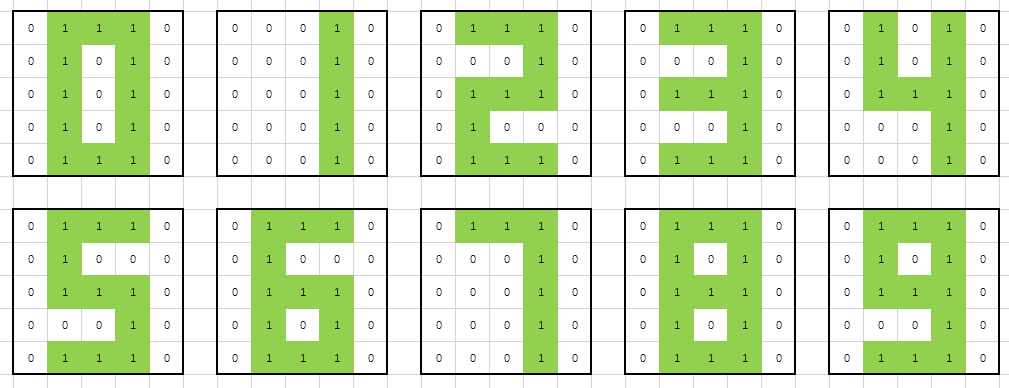
解:
-
因为输出为0~9这10个数字,所以输出有10个神经元;输入为5*5 = 25个像素值,所以输入层有25个神经元。先构建10个感知机分类器,每个分类器只区分是否为某个数字。比如:classifier_1用来区分图像上的数字是否为1,为1则输出1,不是1则输出0。整个神经网络结构如下:
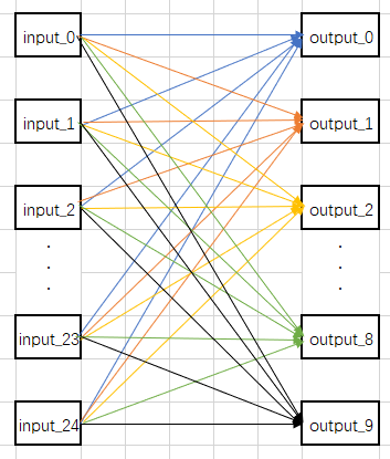
-
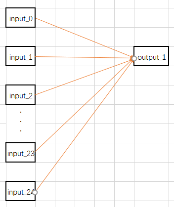
单独拿classifier_1的出来说明感知机计算过程,classifier_1结构如下:
 假设初始化classifier_1的偏置b=0,w=[0,0,…,0](25个0),w转化为5*5像素点的对应关系如下图所示:
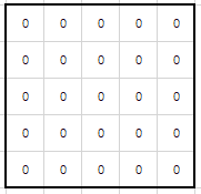
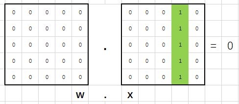
把0~9 这个10个实例分别代入计算 w.x 的值,发现都为0,无法区分图像是否为1。下图是 w.x (1)的计算结果(x (1)表示图像为数字1的实例特征):
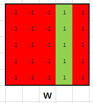
于是计算Loss(Loss越大,表明该模型的参数w越烂),通过反向传递来调整w,如此迭代数次后,可能得到w如下所示(对应数字1的实例,1的位置仍为1,0的位置为-1):
此时 w.x 的值分别为
-
w.x(0) = -2
-
w.x(1) = 5
-
w.x(2) = -3
-
w.x(3) = -1
-
w.x(4) = 1
-
w.x(5) = -3
-
w.x(6) = -4
-
w.x(7) = 3
-
w.x(8) = -3
-
w.x(9) = -2
由此得出偏置b=-5,最后得到classifier_1为:
- 同理可以计算出0~9的所有感知机分类器。最后等到的神经网络可以正确分类这10个数字。
1.3 搭建⼀个简单的分类⼿写数字的⽹络
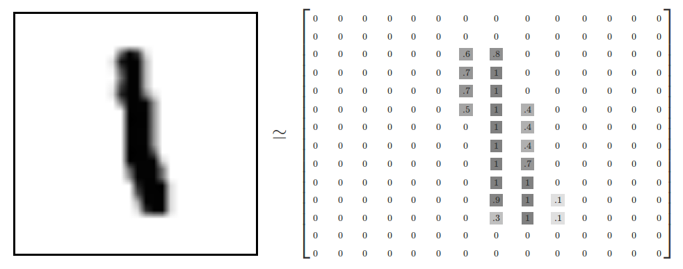
数据来自MNIST,训练数据和测试数据都是一些扫描得到的 28 × 28 的⼿写数字的图像组成,如下图所示:
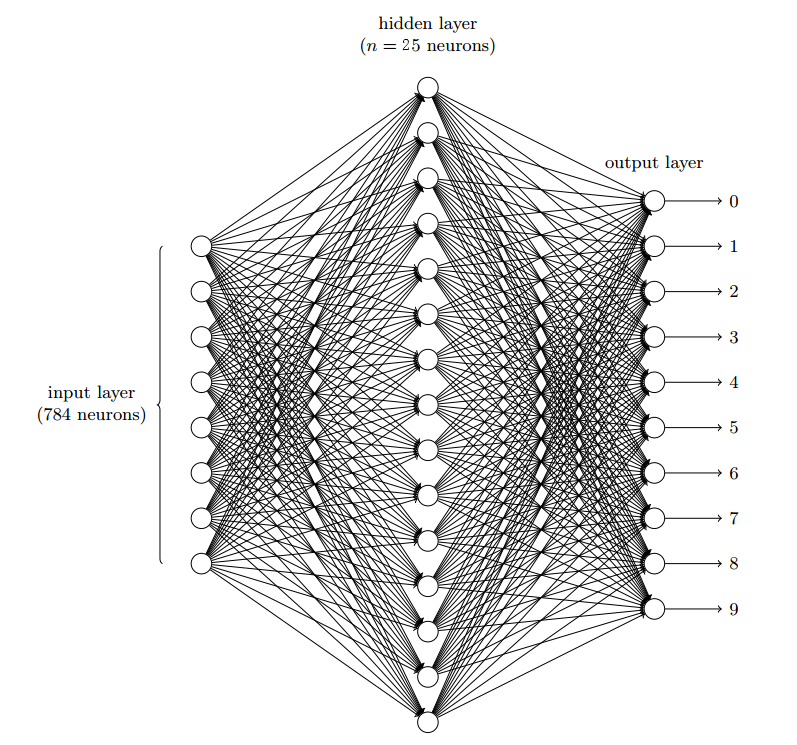
所以输⼊层包含有 784 = 28 × 28 神经元。输出依然为0~9这10个数字,所以输出有10个神经元。设置一个隐藏层,把隐藏神经元为25个。模型如下图所示
输出层到隐藏层大家可以先暂时理解为把一个28 × 28像素的图像,经过感知机运算,变成一个 5 x 5 像素的图形(比如把整个 28 × 28 像素图像 5 x 5 等分,然后判断每个区域是否存在灰度),然后按例1的方法进行数字分类。
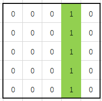
解释:假设隐藏层的第4个神经元只是⽤于检测如下的图像是否存在:

为了达到这个⽬的,它通过对此图像对应部分的像素赋予较⼤权重,对其它部分赋予较⼩的 权重。
同理,我们可以假设隐藏层的第9,第14,第19,第24个神经元是为检测下列图⽚是否存在:
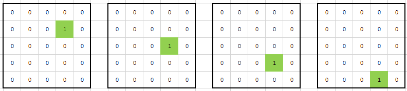
就像你能猜到的,这5幅图像组合在⼀起构成了前⾯例子1中的数字图像中的 1:
如果所有隐藏层只有这5个神经元被激活那么我们就可以推断出这个数字是 1。
1.3.1 构建一个Network 类
下面构建该神经网络,下面这段代码来自https://github.com/mnielsen/neural-networks-and-deep-learning/blob/master/src/network.py,(原来的代码只适合Python2.7,修改后的代码可以在Python3.6上运行,如果Python版本为2.x,请运行原代码,也就是git上的代码。如果Python版本为3.x,可以运行下面版本的代码)
1
2
3
4
5
6
7
8
9
10
11
12
13
14
15
16
17
18
19
20
21
22
23
24
25
26
27
28
29
30
31
32
33
34
35
36
37
38
39
40
41
42
43
44
45
46
47
48
49
50
51
52
53
54
55
56
57
58
59
60
61
62
63
64
65
66
67
68
69
70
71
72
73
74
75
76
77
78
79
80
81
82
83
84
85
86
87
88
89
90
91
92
93
94
95
96
97
98
99
100
101
102
103
104
105
106
107
108
109
110
111
112
113
114
115
116
117
118
119
120
121
122
123
124
125
126
127
128
129
130
131
132
133
134
135
136
137
138
139
140
141
142
143
144
145
146
147
148
149
150
151
152
153
154
155
156
157
158
159
160
161
162
163
164
165
166
167
168
169
170
171
172
173
174
# encoding = utf-8
"""
network.py
~~~~~~~~~~

A module to implement the stochastic gradient descent learning
algorithm for a feedforward neural network.  Gradients are calculated
using backpropagation.  Note that I have focused on making the code
simple, easily readable, and easily modifiable.  It is not optimized,
and omits many desirable features.
"""

#### Libraries
# Standard library
import random

# Third-party libraries
import numpy as np

class Network(object):

    def __init__(self, sizes):
        """The list ``sizes`` contains the number of neurons in the
        respective layers of the network.  For example, if the list
        was [2, 3, 1] then it would be a three-layer network, with the
        first layer containing 2 neurons, the second layer 3 neurons,
        and the third layer 1 neuron.  The biases and weights for the
        network are initialized randomly, using a Gaussian
        distribution with mean 0, and variance 1.  Note that the first
        layer is assumed to be an input layer, and by convention we
        won't set any biases for those neurons, since biases are only
        ever used in computing the outputs from later layers."""
        """参数``sizes`` 是个list,代表每层有个几个神经元
        [784, 25, 10] 表示该神经网络模型有3层:
        	第一层784个神经元,
        	第二层25个神经元,
        	第三层10个神经元"""
        self.num_layers = len(sizes)
        self.sizes = sizes
        self.biases = [np.random.randn(y, 1) for y in sizes[1:]]
        self.weights = [np.random.randn(y, x)
                        for x, y in zip(sizes[:-1], sizes[1:])]

    def feedforward(self, a):
        """Return the output of the network if ``a`` is input."""
        """参数``a`是来自上一层的输入集合;
        	返回结果为该层神经元的输出集合"""
        for b, w in zip(self.biases, self.weights):
            a = sigmoid(np.dot(w, a)+b)
            # print(a)
        return a

    def SGD(self, training_data, epochs, mini_batch_size, eta,
            test_data=None):
        """Train the neural network using mini-batch stochastic
        gradient descent.  The ``training_data`` is a list of tuples
        ``(x, y)`` representing the training inputs and the desired
        outputs.  The other non-optional parameters are
        self-explanatory.  If ``test_data`` is provided then the
        network will be evaluated against the test data after each
        epoch, and partial progress printed out.  This is useful for
        tracking progress, but slows things down substantially."""
        """
        args:
        	training_data 是训练数据集合
        	epochs 是重复训练多少次
        	mini_batch_size	是每次训把训练数据划分成多大的包,来分批训练
        	eta 是学习速率
        	test_data 是测试数据
        """
        if test_data:
            n_test = len(test_data)
        n = len(training_data)
        for j in range(epochs):
            random.shuffle(training_data)
            mini_batches = [
                training_data[k:k+mini_batch_size]
                for k in range(0, n, mini_batch_size)]
            for mini_batch in mini_batches:
                self.update_mini_batch(mini_batch, eta)
            if test_data:
                print("Epoch {0}: {1} / {2}".format(
                    j, self.evaluate(test_data), n_test))
            else:
                print("Epoch {0} complete".format(j))

    def update_mini_batch(self, mini_batch, eta):
        """Update the network's weights and biases by applying
        gradient descent using backpropagation to a single mini batch.
        The ``mini_batch`` is a list of tuples ``(x, y)``, and ``eta``
        is the learning rate."""
        """
        利用梯度下降,更新w,b的
        """
        nabla_b = [np.zeros(b.shape) for b in self.biases]
        nabla_w = [np.zeros(w.shape) for w in self.weights]
        # print('nabla_b:', nabla_b)
        # print('nabla_w:', nabla_w)
        for x, y in mini_batch:
            delta_nabla_b, delta_nabla_w = self.backprop(x, y)
            nabla_b = [nb+dnb for nb, dnb in zip(nabla_b, delta_nabla_b)]
            nabla_w = [nw+dnw for nw, dnw in zip(nabla_w, delta_nabla_w)]
        self.weights = [w-(eta/len(mini_batch))*nw
                        for w, nw in zip(self.weights, nabla_w)]
        self.biases = [b-(eta/len(mini_batch))*nb
                       for b, nb in zip(self.biases, nabla_b)]

    def backprop(self, x, y):
        """Return a tuple ``(nabla_b, nabla_w)`` representing the
        gradient for the cost function C_x.  ``nabla_b`` and
        ``nabla_w`` are layer-by-layer lists of numpy arrays, similar
        to ``self.biases`` and ``self.weights``."""
        """
        反向传递
        """
        nabla_b = [np.zeros(b.shape) for b in self.biases]
        nabla_w = [np.zeros(w.shape) for w in self.weights]
        # feedforward
        activation = x
        activations = [x] # list to store all the activations, layer by layer
        zs = [] # list to store all the z vectors, layer by layer
        for b, w in zip(self.biases, self.weights):
            z = np.dot(w, activation)+b # np.dot() 点积
            zs.append(z)
            activation = sigmoid(z)
            # print(activation)
            activations.append(activation)
        # backward pass
        delta = self.cost_derivative(activations[-1], y) * \
            sigmoid_prime(zs[-1])
        nabla_b[-1] = delta
        nabla_w[-1] = np.dot(delta, activations[-2].transpose())
        # Note that the variable l in the loop below is used a little
        # differently to the notation in Chapter 2 of the book.  Here,
        # l = 1 means the last layer of neurons, l = 2 is the
        # second-last layer, and so on.  It's a renumbering of the
        # scheme in the book, used here to take advantage of the fact
        # that Python can use negative indices in lists.
        for l in range(2, self.num_layers):
            z = zs[-l]
            sp = sigmoid_prime(z)
            delta = np.dot(self.weights[-l+1].transpose(), delta) * sp
            nabla_b[-l] = delta
            nabla_w[-l] = np.dot(delta, activations[-l-1].transpose())
        return (nabla_b, nabla_w)

    def evaluate(self, test_data):
        """Return the number of test inputs for which the neural
        network outputs the correct result. Note that the neural
        network's output is assumed to be the index of whichever
        neuron in the final layer has the highest activation."""
        """
       	用测试数据评估模型准确率;
       	返回 正确数据个数/总测试数据个数
        """
        test_results = [(np.argmax(self.feedforward(x)), y)
                        for (x, y) in test_data]
        # print(test_results)
        return sum(int(x == y) for (x, y) in test_results)

    def cost_derivative(self, output_activations, y):
        """Return the vector of partial derivatives \partial C_x /
        \partial a for the output activations."""
        return (output_activations-y)

#### Miscellaneous functions
def sigmoid(z):
    """The sigmoid function."""
    return 1.0/(1.0+np.exp(-z))

def sigmoid_prime(z):
    """Derivative of the sigmoid function."""
    return sigmoid(z)*(1-sigmoid(z))
1.3.2 处理MNIST 数据
加载 MNIST 数据的代码如下(原来的代码只适合Python2.7,修改后的代码可以在Python3.6上运行):
1
2
3
4
5
6
7
8
9
10
11
12
13
14
15
16
17
18
19
20
21
22
23
24
25
26
27
28
29
30
31
32
33
34
35
36
37
38
39
40
41
42
43
44
45
46
47
48
49
50
51
52
53
54
55
56
57
58
59
60
61
62
63
64
65
66
67
68
69
70
71
72
73
74
75
76
77
78
79
80
81
82
83
84
85
86
87
88
89
90
91
92
93
94
# encoding = utf-8
"""
mnist_loader
~~~~~~~~~~~~

A library to load the MNIST image data.  For details of the data
structures that are returned, see the doc strings for ``load_data``
and ``load_data_wrapper``.  In practice, ``load_data_wrapper`` is the
function usually called by our neural network code.
"""

#### Libraries
# Standard library
import pickle
import gzip

# Third-party libraries
import numpy as np

def load_data():
    """Return the MNIST data as a tuple containing the training data,
    the validation data, and the test data.

    The ``training_data`` is returned as a tuple with two entries.
    The first entry contains the actual training images.  This is a
    numpy ndarray with 50,000 entries.  Each entry is, in turn, a
    numpy ndarray with 784 values, representing the 28 * 28 = 784
    pixels in a single MNIST image.

    The second entry in the ``training_data`` tuple is a numpy ndarray
    containing 50,000 entries.  Those entries are just the digit
    values (0...9) for the corresponding images contained in the first
    entry of the tuple.

    The ``validation_data`` and ``test_data`` are similar, except
    each contains only 10,000 images.

    This is a nice data format, but for use in neural networks it's
    helpful to modify the format of the ``training_data`` a little.
    That's done in the wrapper function ``load_data_wrapper()``, see
    below.
    """
    f = gzip.open(r'..\data\mnist.pkl.gz', 'rb')

    training_data, validation_data, test_data = pickle.load(f,encoding='bytes')
    # f.close()
    training_data = list(training_data)
    validation_data = list(validation_data)
    test_data = list(test_data)
    return (training_data, validation_data, test_data)

def load_data_wrapper():
    """Return a tuple containing ``(training_data, validation_data,
    test_data)``. Based on ``load_data``, but the format is more
    convenient for use in our implementation of neural networks.

    In particular, ``training_data`` is a list containing 50,000
    2-tuples ``(x, y)``.  ``x`` is a 784-dimensional numpy.ndarray
    containing the input image.  ``y`` is a 10-dimensional
    numpy.ndarray representing the unit vector corresponding to the
    correct digit for ``x``.

    ``validation_data`` and ``test_data`` are lists containing 10,000
    2-tuples ``(x, y)``.  In each case, ``x`` is a 784-dimensional
    numpy.ndarry containing the input image, and ``y`` is the
    corresponding classification, i.e., the digit values (integers)
    corresponding to ``x``.

    Obviously, this means we're using slightly different formats for
    the training data and the validation / test data.  These formats
    turn out to be the most convenient for use in our neural network
    code."""
    tr_d, va_d, te_d = load_data()
    training_inputs = [np.reshape(x, (784, 1)) for x in tr_d[0]]
    training_results = [vectorized_result(y) for y in tr_d[1]]
    training_data = zip(training_inputs, training_results)
    validation_inputs = [np.reshape(x, (784, 1)) for x in va_d[0]]
    validation_data = zip(validation_inputs, va_d[1])
    test_inputs = [np.reshape(x, (784, 1)) for x in te_d[0]]
    test_data = zip(test_inputs, te_d[1])
    training_data = list(training_data)
    validation_data = list(validation_data)
    test_data = list(test_data)
    return (training_data, validation_data, test_data)

def vectorized_result(j):
    """Return a 10-dimensional unit vector with a 1.0 in the jth
    position and zeroes elsewhere.  This is used to convert a digit
    (0...9) into a corresponding desired output from the neural
    network."""
    e = np.zeros((10, 1))
    e[j] = 1.0
    return e
1.3.3 运行该代码
1
2
3
4
5
6
7
# encoding = utf-8
import src.mnist_loader as mnist_loader
import src.network as network

training_data, validation_data, test_data = mnist_loader.load_data_wrapper()
net = network.Network([784, 25, 10])
net.SGD(training_data, 30, 10, 3.0, test_data=test_data)
运行结果:
1
2
3
4
5
6
7
8
9
10
11
12
13
14
15
16
17
18
19
20
21
22
23
24
25
26
27
28
29
30
Epoch 0: 5844 / 10000
Epoch 1: 7579 / 10000
Epoch 2: 7676 / 10000
Epoch 3: 7584 / 10000
Epoch 4: 9390 / 10000
Epoch 5: 9483 / 10000
Epoch 6: 9514 / 10000
Epoch 7: 9562 / 10000
Epoch 8: 9547 / 10000
Epoch 9: 9563 / 10000
Epoch 10: 9591 / 10000
Epoch 11: 9591 / 10000
Epoch 12: 9587 / 10000
Epoch 13: 9628 / 10000
Epoch 14: 9622 / 10000
Epoch 15: 9633 / 10000
Epoch 16: 9633 / 10000
Epoch 17: 9610 / 10000
Epoch 18: 9611 / 10000
Epoch 19: 9640 / 10000
Epoch 20: 9639 / 10000
Epoch 21: 9634 / 10000
Epoch 22: 9646 / 10000
Epoch 23: 9641 / 10000
Epoch 24: 9656 / 10000
Epoch 25: 9650 / 10000
Epoch 26: 9644 / 10000
Epoch 27: 9662 / 10000
Epoch 28: 9645 / 10000
Epoch 29: 9650 / 10000
注:如果对函数 backprop (反向传播)部分不理解,点击传送门《反向传播算法如何⼯作》
1.4 代码和环境部署
1.4.1 原代码和环境部署
原代码地址https://github.com/mnielsen/neural-networks-and-deep-learning/blob/master/src/network.py
原代码环境部署请参考https://github.com/mnielsen/neural-networks-and-deep-learning
1.4.2 博主个人代码和环境部署
代码下载地址:https://pan.baidu.com/s/1Q7Ta8aUJ3X_MOfe1nd-rPQ
提取密码:9uxu
该压缩包包含 environment.yaml 文件
代码环境部署:
- 安装Anaconda,安装方式参考:https://blog.csdn.net/ITLearnHall/article/details/81708148
- 运行Anaconda Prompt,输入“conda env create -f {{environment.yaml文件的绝对路径}}”,比如
1
conda env create -f E:\environment.yaml
- 该命令执行完毕后,安装环境就完成了。这时候Python解释器的地址是:C:\Users\用户名\AppData\Local\conda\conda\envs\mlcc_gpu\python.exe,在IDE添加该解释器。